

A Comprehensive Deep Dive to Balancer
A Comprehensive Deep Dive to Balancer

Uniswap’s XY=K formula has been a game-changer for DeFi. In our previous blog post “A Comprehensive Deep Dive into AMMs,” we noted that Uniswap’s formula isn’t the only one employed by Automated Market Makers (AMMs). Different pool types offer distinct benefits, such as reducing slippage rates or facilitating more efficient trades for swappers, and some even assist liquidity providers (LPs) who hold LP tokens as a tool for portfolio balancing. Today, we’re exploring Balancer’s customized pools, which are an extension of the XY=K formula, allowing for the creation of pools with various asset compositions. Our discussion draws from the Balancer whitepaper, and we’ve organized our findings into several key topics:
What was innovative about Balancer
Definition of the value function
Examples of customized pools
How to calculate the price in a customized pool
Proof of constant value distribution
How providing liquidity can balance a portfolio
Efficiency and slippage comparison
Balancer’s formula enables the creation of customized pools, which is a functionality not available with Uniswap’s standard model. For instance, a Uniswap pool is restricted to containing two assets with identical balances. However, Balancer’s formula allows for the creation of pools that can include three, four, five, or more assets, without requiring equal balances. This means that the weights of the assets in the pool are at our discretion. For example, one could design a pool with Ethereum (ETH) and DAI, allocating 80% of the pool’s value to ETH and 20% to DAI.
In contrast, the Uniswap model operates on the XY=K formula, ensuring that the weight balances of assets remain equal. But how does this work? Let’s imagine we have a pool with tokens A and B following the XY=K formula, where X represents the quantity of token A, and Y is the quantity of token B. From our calculations in the blog post about Uniswap V2, we know that when Alice wants to purchase an amount p of token A with token B, the unit price approaches Y/X as p approaches zero. Without any slippage, the price would stabilize at Y/X. Thus, we can define the theoretical price of token A in relation to token B as Y/X. Consequently, since token A’s quantity in the pool is X, its total balance compared to token B is Y. With token B priced at 1 relative to itself, its total balance in the pool is also Y, resulting in the pool’s total value being 2Y when measured against token B. Conversely, the total value is 2X when measured against token A, establishing that the weights of tokens A and B are inherently equal. We will now turn our attention to how Balancer’s formula might alter these weight distributions.Balancer’s value function diverges from the simplicity of Uniswap’s formula. It is expressed as
where
t ranges over the tokens in the pool;
B_t is the balance (or amount) of token t in the pool;
W_t is the normalized weight of the token, such that the sum of all normalized weights is 1.
The logic behind trades is simple with Uniswap’s formula, keeping V constant. Let’s consider some pools generated by the value function:
Two assets with 50–50 weight balance:
Suppose that we want to create a pool consisting of two tokens, namely t1 and t2, with the same weighted balance. Then our formula becomes
It seems familiar right? If we take the square of the two sides we reach
and if we define
we will have
which is the classical constant product formula.
Let’s assume Alice wants to buy p many token 1 (which is t1) and by the formula
she needs q many token 2 (i.e, t2). Which means
however, from this, we have
As a result we have same (p,q) pair working with the both equations effectively. Therefore we can say that Balancer’s value function allows us to create classical pools introduced by Uniswap V2. However we have more pool options.
Three assets with equal weight balance:
Similar to above, if we create a pool consisting of three tokens, namely t1, t2 and t3 with the same weighted balance, then our formula becomes
By defining
we get
which is quite similar to our classical formula. But if we change the weights, our formula becomes slightly different.
Two assets with 80–20 weight balance:
Let’s say we create a pool with an 80–20 weight balance between two assets such that the balance of t1 is 80% where t2’s 20%. Then our formula would be
Similar to above if we define
then we get
The logic is quite easy to understand, but let’s check one more example.
Three assets with 40–40–20 weight balance:
Just like the above examples we have three tokens namely t1, t2 and t3 and their balance is 40–40–20 respectively. If we put in these in to the formula we have:
the move is same: we define
As a result
All of the pool types above have different aspects in terms of their slippage rates. We will investigate all of them in the next paragraphs, however first we need to examine how to calculate the price of an asset in a customized pool with respect to other assets in the pool. As we discussed in the blog post about AMM’s, the price of tokens is highly dependent on the amount of the trade and the liquidity of the pool, see the section related slippage.
Now assume we have a generic pool with created the equation of value function. Let’s say that Alice buys A0 unit token 0 in exchange for Ai unit token i, then the price is Ai/A0. To maintain consistency with the notation used in the whitepaper, let’s define
We call it the effective price. As we know it’s dependent on the values A0, A1 and if these values become smaller, the slippage rate decreases. Then let’s recall our calculus classes and take the limit of the effective price as A0, A1 approach 0.
where ΔB’s representing the change of token amounts of the pool. This limit is simply
In order to handle with this derivative let’s express Bi in the form of B0. In order to do that we need to focus on the value function, which is
Therefore;
We can use it to handle our partial derivative:
and this is equal to
Since
is simply a coefficient, we can factor it out of the derivative.
From now on our task is to just take a basic derivative and calculate the result.
And that’s all, this is our price formula, seems disgusting huh? Don’t worry, we still have some moves to manipulate it. Let’s multiply both the dividend and divisor of the first division with a magical number:
Then we have
Also by using the definition of V we can manipulate the first division:
Finally, we’ve reached a nice expression. This limit is defined as the spot price and denoted
So we have
That means for the relatively small trades with respect to the pool’s liquidity, you can expect the price around that value (excluding the fees).
From now on, we understand the pricing of a token within a pool relative to other tokens. Let’s focus on the weight distributions. At the beginning, we said Balancer’s formula allows us to create specific pools such that 80% of the total value in the pool is of the form ETH and 20% is DAI. In fact, W_t , the normalized weight of the token means the total value of the pool. Let’s say
represents the total value of pool in terms of token t, and
represents the total value of tokens n in terms of t, i.e., how many tokens t the balance of token n is worth it. Our claim is
Let’s begin with the total value of the pool in terms of t.
It is evident that the total value of the pool in terms of t equals the sum of the total values of all tokens in the pool in terms of t. We need to focus on the
Recall that
is the price of token n with respect to token t. Therefore
If we take out B_t, and plug the value of
into the summation above we get:
B_t and W_t are constant so we can take them out. Hence,
by the definition of Wn’s. Therefore, the total value of the pool in terms of t is equal to B_t/W_t. We are almost done. Let’s define Sn as the share of token n in the pool. In order to calculate Sn we need to divide the total value of token n by the total value of the pool. This is given by:
Therefore, the weight balances of tokens in the formula really represent their shares in the pool.
Let’s focus on the practical implications of this fact. Many hedge funds employ a balancing strategy within their portfolio. As the price of one asset increases relative to others, they sell it in exchange for less expensive ones, and vice versa. This tactic prevents any single asset from either dominating or being dominated by the others in the portfolio. Through this process, they capitalize on the gains from the higher-performing assets and bolster their positions in others. Also, maintaining a diverse asset portfolio mitigates the risk associated with reliance on a single asset. In essence, this is an efficient investment strategy.
But how can we apply this strategy to cryptocurrency assets? By becoming a Liquidity Provider (LP) on Balancer. As we have demonstrated, Balancer’s custom pools help maintain asset ratios in line with their prices. For instance, if you wish to balance your holdings of ETH, LQTY, and LUSD equally, providing liquidity to Balancer’s 33LUSD-33LQTY-33WETH pool ensures that each asset in your portfolio maintains equal value. Additionally, you profit from trading fees and potentially from BAL token incentives while maintaining balance in your portfolio.
What if there isn’t a pool that matches your portfolio? There’s no need for concern. With Balancer’s pool creation page, you can easily set up your own pool. The liquidity might start off low. If someone manipulates your pool and it is not re-balanced, you can purchase the necessary assets from the open market to correct it. Essentially, you’ll be engaging in arbitrage with your pool, profiting from the adjustments you make.
Balancer offers significant advantages for liquidity providers. But what about traders? To evaluate swap efficiency in terms of slippage, consider two pools: one follows Uniswap’s constant product model, and the other is a customized pool with two assets weighted at 66.6% and 33.3% such that token A’s weight is 66.6%. We have two formulas:
for the constant product pool, and
for the customized pool. Where, X,Z corresponds the amount of token A and Y,T are of token B. Now let’s assume the price of token A in terms of token B is the same in both pools and the total value of pools are the same. Using these two pieces of information we can write Z,T in terms of X,Y. As we proved above, the value of the first pool is 2X and the second one’s value is 3Z/2 in terms of token A. So,
And similarly,
Therefore our value function becomes;
Now suppose that Alice buys the same amount of token A from both pools. Therefore, slippage — the difference between the real and theoretical price of these trades — is calculated by.
where;
And,
where;
Now we will prove that
which means the Balancer pool containing two weighted assets such that weights are 33.3% and 66.6% is less efficient than the Uniswap’s pool in terms of slippage. In fact, this is not special to 33.3%-66.6% weights. The optimum pool is the 50–50 one. Since the other terms are equal, it’s enough to show that
in order to prove
Let’s begin
coming from the definition directly.
since
we can say that
Thus we have;
By the same argument above,
implies
Therefore, we get
which means
Thus, we have proved that buying token A from the customized pool is inefficient in terms of slippage. Similarly, it can be shown that buying token B is also inefficient regarding slippage. Furthermore, for other customized pools with varying weight balances, the outcome remains consistent. The Uniswap formula, or a customized Balancer pool with equal balances, proves to be more efficient than other configurations. The chart below illustrates the percentage of slippage incurred by a pool with $200,000 worth of assets, composed of tokens A and B, for a trade amount of $1,000 across varying weights of token A. The symmetry around the 50% mark reflects the constant total weight, where the sum of weights for A and B always equals 100%.
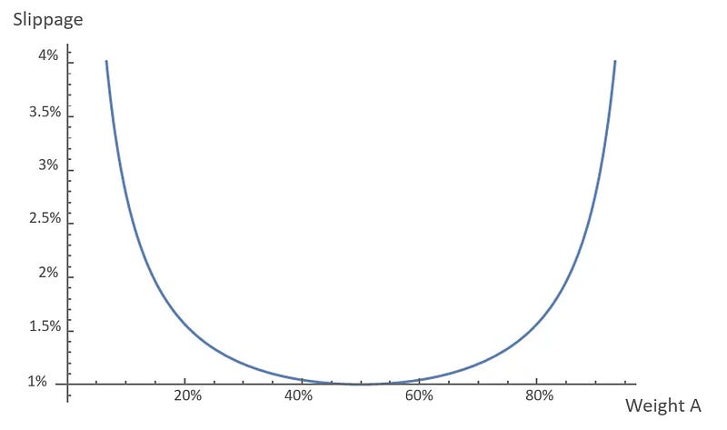
The graph demonstrates that the slippage rate escalates more rapidly as the weight of one asset approaches zero. For this reason, in pools with two assets, it is uncommon for one asset to have a weight less than 20%. Consequently, based on the pool statistics provided, we can assert that the maximum slippage difference between a traditional Uniswap pool and a Balancer pool is approximately 0.5%. It’s important to note that this graph assumes a trade equivalent to 1% of one of the pool’s assets, a significant amount for the average daily trade, given that most pools are valued in the millions. If we consider a smaller trade, say 0.1% of one of the assets — which is still considerable for many pools — the slippage in a traditional Uniswap pool would be around 0.1%, compared to a maximum of 0.15% in Balancer’s. Thus, while transactions in a pool with 50–50 weights are always superior to those in other customized pools, the difference is generally negligible.
We have established that classic Uniswap pools are more efficient, even if the difference is minor for practical purposes. However, Balancer facilitates the creation of pools with more than two assets, which can result in more efficient trading. For example, consider three tokens — token A, token B, and token C — each with a balance of 20,000. If we create three separate pools using the traditional formula, we would have three pools, each with two assets amounting to 10,000 each. In this scenario, when Alice buys 100 units of token A in exchange for token B (the pair is irrelevant since the assets are equally distributed), she would incur a slippage of 1.01%. Now, imagine we create a single pool containing all three assets with equal weights, with each asset contributing 20,000 units. If Bob performs the same transaction as Alice, attempting to buy 100 units of token A in exchange for token B, he would encounter only 0.50% slippage — half that of Alice’s. This reduction is due to the increased liquidity; in essence, Bob’s trade is the same as trading in a classical pool where each asset’s quantity is 20,000. Let’s validate this claim.
We want to show that buying
amount of token A in exchange for token B from both pools that first one is formulated as
and the second one is formulated as
where X,Y,Z represents the balance of token A, token B, token C respectively. Let’s say that
are the price to be paid to the first and second pool respectively. We need to show that they are equal.
Therefore, pools containing more than two assets with equal balances effectively function the same as classical pools with corresponding assets and identical liquidity levels. Thus, it can be said that diversifying the number of assets in a pool, while maintaining equal weights, does not impact slippage, yet the cost of creating such pools decreases significantly. This is evident from the total liquidity not being divided among pools containing only two assets, as illustrated in the earlier comparison between Alice and Bob.
One might question why not simply create a pool with as many assets as possible, given that Balancer V1 allows for up to 8, and V2 allows for 16. Such a pool would presumably concentrate liquidity and facilitate more efficient trades. The overlooked detail in this argument is that liquidity providers cannot contribute liquidity partially. This means that a liquidity provider must own a proportional share of all asset types in the pool. For example, if a liquidity provider holds 0.1% of the LP tokens, they own 0.1% of each of the 16 assets in the pool. Consequently, achieving substantial liquidity is challenging with this approach, as it’s unlikely that LPs will coordinate their actions. Thus, while increasing the number of assets in a pool can bring about some efficiency by tapping into more liquidity, the difficulty of finding liquidity providers with a complete set of tokens increases with the number of asset types.
Numerous interesting outcomes can arise from various pool configurations. For those interested in exploring different scenarios, there is a GitHub repository available. Briefly, I have programmed four JavaScript functions to simulate different swap scenarios. These functions model swaps on a classic Uniswap pool, a customized Balancer pool with two assets at 80–20 weights, a Balancer pool with three assets at equal weights, and another pool with a 40–40–20 weight distribution. The code can be easily modified to examine other scenarios. If you discover something counterintuitive or intriguing, please share it with me so I can include it in this post.
In conclusion, Balancer’s value function lets us set up various types of pools to suit different needs for traders and liquidity providers. This post went into detail about what Balancer offers and how its math works, especially when compared to Uniswap. Thanks for taking the time to read; your engagement with the content is highly valued, and I invite any feedback you might have. Also, don’t forget to follow me on Twitter and subscribe my Substack.